")
")
| Issue |
OCL
Volume 33, 2026
Rapeseed / Colza
|
|
|---|---|---|
| Article Number | 9 | |
| Number of page(s) | 13 | |
| DOI | https://doi.org/10.1051/ocl/2026002 | |
| Published online | 11 March 2026 | |
Research article
Efficient species segmentation throughout the growing season of oilseed rape-service plant intercropping using transfer learning☆
L’utilisation des méthodes de transfer learning permet un découpage efficace des espèces sur des images d’association colza-plantes de services à différents stades
1
Plant-Production Systems, Agroscope, Nyon, Switzerland
2
Ecole Polytechnique Fédérale de Lausanne, Lausanne, Switzerland
3
USC 1432 LEVA, Ecole Supérieure des Agricultures, INRAE, SFR 4207 QUASAV, Angers, France
4
Picterra, Chavannes, Switzerland
* Corresponding author: This email address is being protected from spambots. You need JavaScript enabled to view it.
Received:
26
June
2025
Accepted:
20
January
2026
Abstract
Semantic segmentation methods have become increasingly popular in the field of agronomy for their ability to accurately and efficiently analyse images of crops. These methods use machine learning algorithms to assign semantic labels to each pixel in an image and require extensive amount of labelled data. Currently, most of the available models focus on crop and weed identification and target a single growth stage. In this paper, we propose a robust semantic segmentation method for estimating the dynamics of multi-species cover in intercropping systems, using only 50 images for training the model. We applied transfer learning on the well-established convolutional neural network DeepLab to decrease the image annotation effort. Three models are trained using field images from a three-year field trial with canopy densities ranging from early development at 1.2% to well-developed canopy covers of 98.7%. Overall, we propose a two-class segmentation model to differentiate vegetation from soil, obtaining 96.8% mean accuracy. Two methods for three-class segmentation models to identify soil, oilseed rape and the other plants are proposed, reaching best mean accuracy of 96.2%. The proposed method is able to differentiate oilseed rape from service plant mixtures at all growing stages, allowing for accurate assessment of the dynamic competition for light between these species. Hence, semantic segmentation methods in agronomy have the potential to support study and management of crops, enabling more accurate and efficient data collection and analysis.
Résumé
Les méthodes de segmentation sémantique sont devenues de plus en plus populaires dans le domaine de l’agronomie, grâce à leur capacité à analyser précisément et efficacement les images des cultures. Ces méthodes utilisent des algorithmes de machine learning pour classer chaque pixel de l’image, et nécessitent un grand nombre de données. Actuellement, la plupart des modèles disponibles proposent l’identification d’une culture et des adventices et ne ciblent qu’un seul stade de développement. Dans cet article, nous proposons une méthode de segmentation sémantique robuste permettant d’estimer la dynamique de couverture d’associations complexes de cultures, en n’utilisant que 50 images pour entraîner le modèle. Nous avons utilisé une méthode de transfer learning sur le modèle de réseaux de neurones DeepLab déjà entraîné pour réduire l’effort d’annotation des images. Trois modèles ont été entraînés à partir d’images obtenues dans un essai au champ reconduit trois ans, pendant la période de développement de la culture allant d’une couverture du sol de 1,2 % jusqu’à 98,7 %. Nous proposons un modèle de segmentation en deux classes, qui différentie le sol de la végétation, et obtient une précision moyenne de 96,8 %. Deux méthodes pour des modèles de segmentation à 3 classes, identifiant le sol, le colza et les autres espèces végétales sont proposées, et ont une précision moyenne de 96,2 %. Les méthodes proposées sont capables de différentier le colza des mélanges de plantes de services à tous les stades du développement végétatif, et permettent ainsi une évaluation précise de la dynamique de compétition pour la lumière entre les espèces. Ainsi, les méthodes de segmentation sémantique peuvent contribuer à l’étude des associations de cultures et être utilisées dans des outils d’aide à la décision, car elles simplifient et rendent plus précise la collecte et l’analyse des données.
Key words: Image analysis / deep learning / semantic segmentation / intercropping / multi-specific mixtures
Mots clés : Analyse d’image / deep learning / segmentation sémantique / cultures associées / mélanges plurispécifiques
Contribution to the Topical Issue: “Rapeseed / Colza”.
© A.A. de Jong et al., Published by EDP Sciences, 2026
 This is an Open Access article distributed under the terms of the Creative Commons Attribution License (https://creativecommons.org/licenses/by/4.0), which permits unrestricted use, distribution, and reproduction in any medium, provided the original work is properly cited.
Highlights
Segmentation models were developed to detect crop, soil and service plant mixtures vegetation on images taken in the field
These models gave satisfactory results at all stages of vegetative growth despite the limited number of 50 images annotated
It could be a powerful and low-cost tool to analyse the dynamic of complex mixtures like oilseed rape- service plants intercropping
1 Introduction
Since the second half of the 20th century and the Green Revolution, crop production has largely relied on the use of synthetic pesticides and fertilizers (Tilman et al., 2002). The intensive use of these products can lead to negative environmental and health impacts (Tilman et al., 2001; Kim et al., 2017). To cope with the World’s population growth and climate change while mitigating competition for natural resources, agriculture must adopt more sustainable practices maintaining high yields in the upcoming years (FAO, 2017; Martin-Guay et al., 2018). Therefore, interest has grown to develop and apply knowledge about agroecological practices to produce food and plant products. In particular, intercropping systems can enhance grain yield while reducing the reliance on pesticides and synthetic fertilizers (Bedoussac et al., 2015; Brooker et al., 2015; Li et al., 2014; Verret et al., 2017; Dowling et al., 2021). It consists in growing two or more crop species simultaneously in the same field, during at least a part of its growing cycle (Vandermeer et al., 1998). This practice can involve a high number of species (Wendling et al., 2019; Finney et al., 2017), resulting in complex systems to study by researchers and to manage by farmers. Having quick, easy to use and non-destructive methods to study these systems could greatly contribute to i) better understand dynamic processes of the plant-plant interactions in intercropping arrangements, ii) help to conduct large scale participatory investigations about intercropping practices or iii) be used as an indicator to design decisions rules for farmers and extensionists.
During early growth stages, the distribution of light access among the plants species impacts both crop species and weed growth (Midmore, 1993). The canopy cover of the intercrop system is a good indicator of the degree of light competition and hence competition with weeds (Cadoux et al., 2015). Different methods exist for quantifying infield ground cover: i) visual estimation, ii) light measurements above and below the plant cover and iii) image analysis. Visual estimation is time consuming and prone to subjectivity (Büchi et al., 2018). Light measurements are highly sensitive to small variations in illumination and require expensive equipment (Chopin et al., 2018). Image analysis gives objective, non-destructive and more consistent results for infield measurements (Hartmann et al., 2011). Among this method, semantic segmentation assigns a class to each pixel of an image, providing an accurate map for ground cover estimation (Hamuda et al., 2016). Compared to the other available methods, multiclass segmentation enables the identification of species among the vegetation cover (Wang et al., 2019). Hence, this method captures better information to test ecological processes such as facilitation, niche complementarity and competition in intercropping systems. Infield implementation of such method suffers from the outdoor illumination conditions and the overlapping of the leaves at different development stages (Chopin et al., 2018).
Image analysis is among the most popular approaches for phenotyping tasks in agronomy and ecology (Lobet et al., 2013). Typical methods for the image-based canopy cover estimation include color index-based segmentation, threshold-based segmentation, and learning-based segmentation (Wang et al., 2019). Color indexes are combinations of the red-green-blue (RGB) image color bands. Index threshold method divides a color space, transformations such as excess green index (ExG), hue-saturation-value (HSV) and LAB color space (Robertson, 1977), according to dynamic or fixed threshold value. Both methods are simple and quick to implement, providing good results under standard exposure and illumination (Wang et al., 2019). However, they usually require manual adjustments and are not robust under strong illumination conditions (Hamuda et al., 2016). Tuned for detecting green vegetation, their performance decreases greatly when confronted to complex vegetation cover containing yellowing leaves, flowers or colored stems. To overcome these limitations, learning-based methods use machine learning approaches to extract color, shape and texture features (Hamuda et al., 2016b). Although these techniques involve more computational effort compared to the unsupervised ones, they remain better choice for canopy cover estimation (Sadeghi-Tehran et al., 2017).
When dealing with semantic segmentation problems, deep learning methods outperform classical learning techniques such as support-vector machine (SVM), Random Forest, and K-means Clustering (Aitkenhead et al., 2003). Deep learning methods rely on a Fully Convolutional Network (FCN), which process images through successive layers designed to automatically extract relevant visual features. Convolutional layers apply small filters that slide over the image to detect local patterns such as edges, textures, or shapes, progressively capturing more complex features. Pooling layers reduce the spatial resolution of the feature maps, which decreases the data size, limits sensitivity to small spatial variations, and helps the model focus on the most informative features. Fully connected layers, usually placed at the end of the network, combine all extracted features to produce the final classification or segmentation output. (Long et al., 2015). Lottes et al. (2017) adopted an encoder-decoder structure to improve robustness of canopy pixel classification under high variation in canopy cover density, visual appearance, and soil type. The encoder corresponds to the down sampling part of the network, where the image resolution is gradually reduced while feature complexity increases. The decoder performs the opposite operation by up sampling the encoded features to recover the original image resolution and generate pixel-level predictions. This bottleneck approach enables features learning at multiple scales and ensures generalization. Chen et al. (2018a) introduced further improvement to semantic image segmentation by implementing an encoder-decoder network with dilated separable convolution, which allow the network to capture broader contextual information without increasing the number of parameters or losing spatial resolution. This improves segmentation results on object boundaries and generates excellent performance on PASCAL VOC 2012 (87.8% mean intersection over union (IoU), a metric evaluating the share of overlapping area between the prediction and the target reference) and Cityscapes (82.1% mean IoU) datasets. However, compared to traditional machine learning approaches, convolutional network is laborious to implement due to its high computational power requirement and the need to access large labelled datasets This is especially true for semantic segmentation, which requires time-consuming pixel-level annotations, making it considerably more labor-intensive than tasks such as image classification or object detection.
Transfer learning solves the need of using vast labelled datasets by fine-tuning the weights of a pre-trained network for a new task. This method permits to use a limited amount of data while achieving satisfying performance (Olivas et al., 2009). In recent years, scientists adopted this technique to segment crops accurately in the presence of weeds (Abdalla et al., 2019; Munz and Reiser, 2020), especially for crops and weeds differentiation (Bosilj et al., 2020; Wang et al., 2020). For instance, Abdalla et al. (2019) using transfer learning achieved an accuracy of 96% and 88% of IoU for oilseed rape and weeds segmentation, respectively. Moreover, they showed that data augmentation plays a key role to improve the accuracy and to decrease the training time. In addition, Wang et al. (2020), investigated color space transformation for model robustness against different light conditions of an encoder-decoder deep learning network for crop/weed semantic segmentation. Even though, no improvement was observed for enhancement on RGB images, they achieve satisfying results on the oilseed rape dataset with a mean accuracy of 96% and mean IoU of 89% (Wang et al., 2020).
Despite the importance of competition dynamics in the study of plant communities, most studies are tuned for a specific growth stage. Semantic segmentation of weeds in oilseed rape fields proposed by Bosilj et al. (2020), You et al. (2020), Wang et al. (2020) and Ullah et al. (2021) only targets early stages of the crop development, where the vegetation cover does not exceed 30%. Abdalla et al. (2019) focused on high density vegetation cover, over 80%.
While many published studies proposed efficient approaches for weeds and crops segmentation, including oilseed rape fields (Abdalla et al., 2019; Wang et al., 2020; You et al., 2020; Ullah et al., 2021; Sodjinou et al., 2022), only a few studies tackle species identification in intercropping systems and rarely deal with more than two crop species (Munz and Reiser, 2020; Skovsen et al., 2021). An example of multi-species segmentation given by Skovsen et al. (2021) implements a two-step cascade semantic segmentation to map first four classes grass/clovers/weeds/soil on densely vegetated forage covers, then differentiates red clovers from white clovers, reaching a mean IoU of 68.4%. On a pea and oat intercropping systems, Munz and Reiser (2020) assessed performance of transfer learning on crop species and weeds segmentation at different density cover levels. As a result, training the model on all growth stages increases robustness of the model but decreases the prediction results in some of the single dataset. They achieved a mean IoU of 81%, 80% and 66% on low, intermediate, and high soil cover, respectively. Thus, to precisely study dynamics of intercrop covers, a more accurate multi-species semantic segmentation approach that is reliable over all stages of soil covers is still to be developed.
Therefore, this study proposes a robust semantic segmentation method to accurately estimate multi-species covers dynamics and differentiate oilseed rape from service plants. These intercropping arrangements consist in growing winter oilseed rape as a cash crop with frost sensitive services plants that are grown for contributing to weed control (Lorin et al., 2015; Verret et al., 2017). Farmers in Switzerland who practice this technique use a mix of service plants ranging from 4 to 10 different species (Baux and Schumacher, 2019). Studying the functioning of such cover is challenging and could benefit from image analysis in order to assess the proportion of each crop. The aim of this work is threefold:
Develop an accurate semantic segmentation method for complex vegetation covers of in-field images.
Ensure consistency of the method’s performance at all vegetation development stages.
Provide a tool for the assessment of competition dynamics for light within intercropping systems.
2 Material and methods
In this paper, we propose a two-class semantic segmentation model to differentiate vegetation from soil. Furthermore, we studied two methods for three-class segmentation models to identify soil, oilseed rape and the other plants. The performances of the developed methods were evaluated by comparing to manually annotated images of oilseed rape intercropped with multiple service plant species, known as ground truths.Experimental Design
For the training and the evaluation of the model, images were gathered from several agronomic experiments in western Switzerland. The agronomic and ecological aspects of this study was investigated in other studies (Bousselin, 2022; Bousselin et al., 2024). These experiments were located in Changins (46°23'45.N, 6°15'30.E) and Moudon (46°40'45.N, 6°48'52.E) in 2018, and in Changins in 2019 (46°24'04.N, 6°15'29.E) and 2020 (46°23'46.N, 6°14'05.E).Within these experiments, pure oilseed rape (Brassica napus L. cv. Avatar) and 21 different treatments made of winter oilseed rape intercropped with frost sensitive service plants were used (Tab. S1). Oilseed rape and service plants were respectively sown at row distance of 50 cm and 15 cm. Each intercropping or pure oilseed rape control were allocated on 8 m × 6 m plot with three replicates. In each plot of the Changins site, two subplots of 1 m2 were defined and one was hand weeded and the other one was non-weeded. Only a non-weeded subplot was determined in Moudon.
The service plant mixtures intercropped with oilseed rape included 2 to 7 service plant species (Tab. S1). These intercropping arrangements have been chosen as it often includes a high number of species with contrasted traits (Baux and Schumacher, 2019). The species were based on the predominant species used in Swiss mixtures such as: niger (Guizotia abyssinica (L.f) Cass), buckwheat (Fagopyrum esculentum Moench cv. Lileja), grass peasha (Lathyrus sativus L. cv. Merkur), common vetch (Vicia sativa L. cv. Omiros), lentil (Lens culinaris Medik. cv Red flash), berseem clover (Trifolium alexandrinum L. cv. Winner) and faba bean (Vicia faba L. cv. Fanfare). Additionally, the mustard (Sinapis alba L. cv. Pirat), summer oilseed rape (Brassica napus L. cv. Jumbo-00) and the radish (Raphanus sativus L. cv. Defender) was included each in one treatment (Tab. S1).
Specific attention was carried on intercropping containing buckwheat as this species flowers early and has red stems, which challenges common vegetation segmentation models.
2.1 Image acquisition
Images were taken on each experiment during the fall growing period. Five dates ranging from 18 to 61 days after sowing depending on the site-year (Tab. S2). RGB images were captured using a high-resolution digital mirrorless camera, Canon EOS M10 at a focal length of 15 mm using the kit lens (CANON, EF-M 15–45 mm f/3.5-6.3, Tokyo, Japan) in 2018 and 2019 and Canon EOS M100 with the same lens and settings in 2020. The camera was oriented to the ground fixed at 1.3 m on a horizontal pole attached to a tripod structure. The images were acquired in 2018, 2019 and 2020 with horizontal and vertical resolution of 180 dpi at the corresponding dimensions: 2912 × 5184, 3456 × 5184, and 4000 × 6000 pixels. The plant density cover ranged uniformly from the first sprouts at 1.2% mean vegetation cover to a maximum mean vegetation cover of the intercropping systems at 98.7%.
2.2 Data preparation
2.2.1 Images processing
All ground images were cropped at 0.5 m × 1 m area centered on an interrow taking up to the middle of both adjacent oilseed rape rows (sown at 0.5 m). This configuration was adopted to focus on the development of service plants throughout the studied period. Specific attention was given to crop images keeping the same aspect ratio for the different existing resolutions in the captured images. The dimensions of the resulting images were: 1680 × 2820, 1416 × 2376, and 1945 × 3264 pixels. Additionally, the image resolution was downscaled to save training time. This also permits to remove noise from the images while keeping sufficient information for the semantic segmentation tasks. The images were resized to 1120 × 1880 pixels using PIL resize function with nearest neighbour method (Umesh, 2012), resulting in a horizontal 0.45 mm/pixel and vertical 0.53 mm/pixel resolution. Furthermore, the maximum size of the model inputs is limited by the available GPU memory of the computer. Consequently, the resized images were split into 16 sub-images of 280 × 470 pixels to feed to the model.
2.2.2 Images annotation
Supervised machine learning model depends on labeled dataset of images with corresponding masks of the expected class. Creation of such dataset is determinant thereafter as it sets the ground-truth reference to assess the performances of the model. Since crops and other plants on the images typically have irregular shapes, the annotation step involves considerable efforts and time. To accelerate this process, a two-stage method was implemented to label images as background vegetation class. First, most of the green shades were retrieved using a threshold on the LAB colour space (McLaren, 1976). Then, the missing vegetation areas were manually filled with ImageJ’s (Schindelin et al., 2012) freehand selection tool. A two-class dataset of 160 images was obtained using this method. Half of these images were further manually annotated identifying oilseed rape from the rest of the retrieved vegetation cover, forming a three-class, background-other plants-oilseed rape, dataset of 80 images. Annotation of one image took from 20 to 90 min of work limiting the number of images to be annotated. Hence, this highlights the necessity of adopting transfer learning for this study1.
2.2.3 Data augmentation
By adopting transfer learning, the number of images to annotate is decreased, avoiding substantial labeling effort (Fig. 1). Deep learning models rely on large amount of data to have satisfactory performance. Data augmentation can increase the variety of training samples and prevent overfitting of the model (Takahashi et al., 2019; Bosilj et al., 2020; Su et al., 2021). Conventional data augmentation consists in applying a set of transformations in either data or feature spaces to produce a new set of annotated images. Although Pytorch (Paszke et al., 2019) includes data augmentation implementation within its model pipeline, we used Imgaug (Jung et al., 2020) offering more options. This library enables to register a succession of rules to produce N new images from a reference image. N corresponds to the amount of new images to be created. In this study we set the following rules: every time respectively 50% and 20% of the N images were horizontally and vertically flipped, sometimes they were cropped from −5% to 10% or rotated from −45 to 45 degrees and they could additionally have gaussian blur, brightness values changed, contrasts improved or worsen, and go under perspective transformation. After data augmentation, five new images with ground-truth masks for each training images were produced.
2.3 Model architecture
Image segmentation tasks have long stood at the heart of computer vision challenges (Deng et al., 1999; Yanowitz and Bruckstein, 1989). For this study, we use the well-established DeepLab model for semantic segmentationThis architecture effectively handles dense and heterogeneous vegetation patterns and preserves sharp boundaries, which is critical for complex field images. Its availability in PyTorch also facilitates reproducibility. DeepLab consists of a convolutional neural network composed of two phases: an encoding and a decoding phase (Fig. 2). Neural networks are defined by a succession of node layers connected by weights and thresholds (Gu et al., 2018).
Convolution neural networks comprise convolutional, pooling and fully connected layers. Convolution layers apply a moving filter, or kernel over the input layer to extract features. This process is known as convolution. Pooling layers conduct dimensionality reduction. Fully connected layer occurs when each node in the output layer connects directly to a node in the previous layer. In the DeepLab model, the encoding phase extracts essential information from the image and the decoding phase reconstructs the output of size matching the input image’s one.
DeepLab improves segmentation models such as ResNet (Wu et al., 2019) by using new encoding architecture (Chen et al., 2018b). In fact, DeepLab proves to better deal with dense prediction tasks through upsampled filters, or ‘atrous convolution’, handle objects at multiple scales by using atrous spatial pyramid pooling (Chen et al., 2017) and capture sharper object boundaries (Chen et al., 2018a).
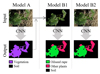 |
Fig. 1 Transfer learning flowchart. The DeepLab model is trained on 200,000 images to predict 21 categories. The learned parameters (in orange) are used to initialize the model training, and the last layer (in blue) is adapted to predict 3 categories (oilseed rape, other plants and soil). Our model input consists of 50 manually labelled images. |
2.4 Model training
For this study, three training processes were drawn. Depending on the task, these processes are split into two categories: training a model A for a two-class segmentation of vegetation from background pixels and training two models B1 and B2 predicting three classes: background, service plants and oilseed rape. Both models A and B2 take as inputs the images produced by the data preparation while model B1 takes as inputs images where the soil pixels are masked (Fig. 3). Following cascading process, model B1’s inputs are generated from model A’s outputs. The goal of this method is to try to force the focus on differentiating service plants from oilseed rape given only the vegetation coverage as information.
Therefore, 100 images were used to train model A and 50 to train models B1 and B2. For each training session, 80% of the images were used for training and 20% for validation, to monitor the model performance on unseen data. To ensure consistency of the results, each experiment was implemented three times using the same parameters. Images were randomly shuffled before each epoch to support stable convergence. Due to GPU limits (∼6 GB VRAM), images were split into patches and a batch size of 2 was used. We tested freezing the backbone and full fine-tuning, with the latter giving the best results. Models were trained for 20 epochs using a fixed learning rate, cross-entropy loss, and Adam optimizer. Training and validation losses were monitored to ensure convergence and prevent overfitting. The total training time was less than 10 h.2
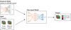 |
Fig. 2 DeepLabv3+ proposed by Chen et al. (2018a) extends DeepLabv3 by employing a encoder-decoder structure. The encoder module encodes multi-scale contextual information by applying dilated convolution at multiple scales, while the simple yet effective decoder module refines the segmentation results along object boundaries. |
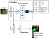 |
Fig. 3 Presentation of the three training workflows of the segmentation models presented in this paper. Model A: two-class segmentation model, Model B1: three-class segmentation model with cascade training method and model B2: three-class segmentation model with direct training methodIn this study, DeepLab model (Chen et al., 2018b) with a ResNet-101 backbone (Wu et al., 2019) trained on COCO 2017 dataset (Lin et al., 2014) of 21 classes is used to train the three models. The final layer of the pretrained model was modified to predict either 2 or 3 categories, depending on the task. Transferring the weights of a semantic segmentation model trained on vast dataset to retrain the models permits to fine-tune the models for a new task with a minimum number of images, which also accelerates convergence during training. |
2.5 Evaluation metrics
To enable fair comparisons between existing methods, evaluation must use standard and well-known metrics. Those metrics are the accuracy and the mean intersection over union (mIoU). The accuracy (Eq. 1) reports the share of pixels in the image which are correctly classified.
 (1)
(1)
Per-class accuracy essentially consists in evaluating a binary mask. True positive (tp) and false positive (fp) are the number of pixels respectively correctly or wrongly predicted to belong to the given class. True negative (tn) and false negative (fn) are the number of pixels respectively correctly or wrongly identified as not belonging to the given class. Accuracy is the sum of tp and tn pixels over the total number of pixels. When a class representation is small within the image, the maximum amount of pixels found as tp will be much smaller than the tn, reporting how well negative case is performing. In this case, the accuracy could provide misleading results.
The intersection over union (IoU) (Eq. 2) quantifies the ratio between the intersection and the union of two sets, in our case the ground truth and our predicted segmentation. The IoU is computed for each class separately and then averaged over all classes, providing the mIoU of the semantic segmentation prediction.
 (2)
(2)
The f1-score (Eq. 3) is the harmonic mean of precision and recall, considered a better indicator of a classifier’s performance than accuracy for this study as it compensates for uneven class distribution in the training dataset.
 (3)
(3)
The precision (Eq. 4) represents the share of pixels classified as vegetation that belongs to the vegetation class.
 (4)
(4)
The recall (Eq. 5) evaluates the share of pixels correctly assigned to a class.
 (5)
(5)
In this paper, global accuracy and mIoU are reported for each models to allow for comparison with the literature. The f1-score is used for describing results of specific cases as it can be explained by how a class perform in term of recall and precision.
The model segmentation performances on images with complex covers was assessed by grouping images based on three categories of sown mixture: oilseed rape monocrop (Mono), oilseed rape intercropped with mix of service plants without buckwheat (Inter) and oilseed rape intercropped with mix of service plants containing buckwheat[CE1] (InterBw) (Fig. 4).
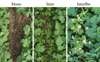 |
Fig. 4 In field images of each sown mixtures type. Monocrop, intercropped oilseed rape with mix of services plants without buckwheat or with mix of services plants containing buckwheat. All images are cropped at 1 m × 0.5 m and taken in Changins, October 7th 2019. Mono: Monocrop, Inter: intercropped oilseed rape with mix of services plants without buckwheat, InterBw: intercropped oilseed rape with mix of services plants containing buckwheat. (Tab. S1 for detailed species composition of Mono, Inter and InterBw) |
3 Results
3.1 Global performance
The two-class segmentation, model A, was trained on 100 in-field images with vegetation densities ranging from early development at 1.2% to well-developed canopy covers of 98.7%. Half of these images was further annotated to produce the three-class dataset for models B1 and B2 where the mean pixels distribution per image between oilseed rape and other plant classes was 36.2% and 19.3%, respectively (Tab. 1; Fig. 5).
All three models demonstrate high performance for their pixel classification task, with respective mean accuracy and mIoU of 96.8% and 90.6% for the two-class model A (Tab. 2), 95.5% and 78.7% for the cascade three-class model B1 and 96.2% and 83.0% for the direct three-class model B2 (Tab. 3). Model A accurately assigns pixels to soil and vegetation classes with both precision values over 95%. Furthermore, the pixels classified as vegetation more often test positive than the ones found as soil class with class recall of 96.0% compared to 93.5% (Tab. 2). Although B2 model performed better than B1 model, both soil and oilseed rape classes were accurately predicted by the three-class models with mean precision exceeding 90%. While the averaged precision of the other plants class was close to 65% both for B1 and B2 (Tab. 3). The three-class models did not predict the other plants class as well as the two others present on the image. Additionally, the high standard devisation for the f1-score on the other plants presented the variability in the performance of the models from one image to the other for the segmentation of the other plants category (Tab. 3).
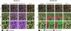 |
Fig. 5 Low, intermediate, and high vegetation coverage field images with respective groundtruth3, prediction and error. On the left, the two-class segmentation model A and on the right, the three class segmentation model B2. LC: low coverage, IC: intermediate coverage and HC: high coverage. In field images of oilseed rape sown with service plants containing buckwheat (InterBw), cropped at 0.5 × 0.5 m. |
Pixel distribution for each testing dataset of the two-class and three-class segmentation models. Mean pixel class share of the N images with standard deviation for each testing dataset of the two-class and three-class segmentation models. Mono: monocrop, Int: intercropping systems without buckwheat, InterBw: intercropping systems with buckwheat, N: number of images per subset, OSR stage: oilseed rape growth stage based on the BBCH scale (Lancashire et al., 1991).
Mean accuracy, mIoU, precision and recall of the 60 test images with standard deviation for vegetation, soil of the testing dataset for the two-class segmentation model. mIoU: mean intersection over union.
Mean accuracy, mIoU, precision and recall of the 30 test images with standard deviation for oilseed rape, service plants and, soil of the testing dataset for three-class segmentation models. mIoU: mean intersection over union.
3.2 Complex intercrop covers
As a result of intercropping, the mean vegetation coverage was higher, with 58.1% and 55.2%, respectively, compared to 44.4% in average for Mono (Tab. 1). Also, the images of monocrop showed higher oilseed rape coverage than the ones in intercropping systems: in average 42.3%, 35.9% and 26.9% for Mono, Inter and InterBw (Tab. 1).
As the corresponding overall f1-scores of Mono, Inter and InterBw reached respectively 97.8%, 96.9% and 95.8% for model A, 97.0%, 92.0% and 90.9% for model B1, 97.2%, 93.6% and 92.5% for model B2. The three models performed better on less complex cover.
The two-class segmentation model demonstrated consistency in predicting the vegetation class over the three sowing mixtures, with vegetation f1-score maximum gap of 1% from 95.1% to 96.1% (Fig. 6). The vegetation class obtained similar precision over the three sowing mixtures. The highest recall was computed on the monocrop dataset scoring at 97.5%, wich is 1.6% to 2.9% more than Inter and InterBw. Both direct and cascade three-class segmentation models accurately predict oilseed rape and background classes. The oilseed rape class was better predicted on the monocrop images than the intercropping systems ones as model B1, model B2 f1-scores respectively achieved 92.7%, 95.7% on Mono. subset, 85.6%, 91.1% on Inter. subset and 85.8%, 89.2% on InterBw subset (Fig. 6). Both models predicted more accurately the other plant class on intercrop without buckwheat than with and perform poorly on monocrop images.
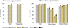 |
Fig. 6 Comparison of the model’s f1-score over the three sown mixture types. The two-class (left) and three-class (right) segmentation models. Sown mixtures mean f1-score of the N images (Tab. 1). Error bars represent the standard deviation. Mono: monocrop, Inter: intercropping systems without buckwheat, InterBw: intercropping systems with buckwheat. |
3.3 Dynamic covers
Two testing dataset arrangements were created to investigate robustness of the models over the full growing season of oilseed rape. First, the testing images were split into three groups of vegetation coverage level: low coverage (LC, <35%), intermediate coverage (IC, between 35% and 65%) and high coverage (HC, >65%) (Tab. 1). Both oilseed rape and other plants coverage increased with the increase of the global vegetation coverage (e.g., mean oilseed rape coverage was 9.4%, 35.4% and 55.1% for LC, IC and HC).
Secondly, the testing dataset was rearranged according to the oilseed rape’s development stages using the BBCH scale (Lancashire et al., 1991), ranging from 12 to 18.
3.4 Vegetation coverage
The two-class segmentation model mean accuracy varied from 97.6% to 96.0% with the increase of vegetation coverage. The decrease of performance from low to high coverage was more pronounced in the three-class segmentation models where mean accuracy of model B1 and B2 respectively ranged from 92.8% to 97.8% and 94.3% to 98.0%. The trend of the models reversed when examining its metrics for the classes of interest: vegetation or service plant and oilseed rape classes. Indeed, the f1-score of LC (91.0%) was lower by 5.9% and 6.5% than the ones of IC (96.9%) and HC (97.5%), respectively (Fig. 7). Furthermore, even though f1-scores of other plants and oilseed rape on HC was higher than the ones on LC. They reach their maximum per-class values on IC (Fig. 7).
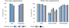 |
Fig. 7 Comparison of the model’s f1-score over three canopy coverage levels. The two-class (left) and three-class (right) segmentation models. Canopy covers mean f1-scores of the N images (Tab. 1). Error bars represent the standard deviation. LC: low cover, IC: intermediate cover and HC: high cover. |
3.5 Oilseed rape development stages
Performance of the two-class and three-class segmentation models slightly decreased with oilseed rape development stage. For instance, mean accuracy of growth stage 12 and 18 shifted from 98.7% to 96.5% model A, 98.5% to 93.3% model B1 and 98.9% to 94.8% model B2. The vegetation class was well predicted on all growth stages, except at very early stage 12, where the f1-score decreased to 88.7%, also showing the lowest recall of 87.1% on this class (Fig. 8). A similar trend was observed on the three-class segmentation models where B1 and B2 f1-score of oilseed rape class were respectively 67.7% and 86.5%, with lowest recall on the class, 55.2% and 80.3% (Fig. 8). In addition, the three-class models performances were lower on the other plant class at stages 12 and 18 with respective f1-scores of 33.8% and 46.5% model B1, 35.6% and 55.5% model B2, also accompanied by a decrease of the recall. With lower standard deviation and more consistent performance, the direct training method, model B2, showed more robustness on oilseed rape class at the different development stages.
4 Discussion
In this study, three semantic segmentation models for the detection of vegetation, soil, and other plants in complex intercropping systems reached high performances. Our results suggest that the two-class segmentation model was highly effective at classifying pixels in field images as either vegetation or soil, with high accuracy on all test datasets. Both three-class segmentation models achieved good performance in classifying soil and oilseed rape. However, the models produced lower accuracy for the other plant class, which may be due to the wide variety of plant species with similar visual characteristics and their lower predominance compared to the two other classes on the images. Similar trends were observed by Kottelenberg et al. (2026) that assessed the ability of CNN models to separate green pixels between cereals, faba bean and weeds in intercropping systems. They observed a lower quality of prediction for weed than for cereals and faba bean that were more dominant and homogenous in the training set of images.
To improve differentiation of oilseed rape from other plants in complex vegetation covers, a cascading method was investigated. This approach tended to perform worse than the model directly retrained from scratch. Nonetheless, our models demonstrated satisfying results on complex intercrop covers, with higher vegetation recall on the Mono dataset and better retrieval of the soil class in the absence of service plants.
Our two-class and three-class segmentation models globally performed better on the Mono dataset. One reason could be that the presence of service plants in the sown system generates variability in the shapes and colours of the vegetation cover. Features are more easily learned by the model when the class is more homogeneous. This could also be explained by the fact that the field images used in this study were centered at the oilseed rape inter-rows, where the service plants are sowed. In absence of service plants, the soil area tends to be covered by oilseed rape leaves whereas, in the intercropped systems, the soil region is scattered by the service plants growing at the inter-row. Because most of the errors occurs at the border of a shape, the model faces difficulty to accurately detect the small patches (Fig. 2). This finding is consistent with previous studies by Abdalla et al. (2019) and Munz and Reiser (2020), which also found that fine-tuning models tend to perform better on simpler, more homogeneous vegetation covers. The three-class segmentation models better detected the other plant class on images with service plants, suggesting that the model lacks the capability to estimate small patches of weeds when most of the vegetation cover is composed of one crop. The issue comes from unbalanced class distribution. To address this, higher weights can be assigned to the other plant class during model training (Phan and Yamamoto, 2020).
Our models also demonstrated consistency over the whole growing season, with the two-class segmentation model performing well even on high vegetation coverage. However, the three-class segmentation models were more successful on intermediate coverage datasets and accurately predicted oilseed rape pixels from BBCH stage 14 to 18.
Compared to the well-established methods, our proposed three-class direct segmentation model performs well on more complex systems, although we acknowledge that our study presents more complex vegetation canopy and is not fine-tuned for a specific growth stage. For instance, our model outperforms the results presented by Munz and Reiser (2020) on pea/oat intercropping systems, although they used only images of sole crops for training the networks and their dataset covers a smaller range of canopy coverage (from 4% to 52%). Furthermore, Wang et al. (2020) only focused on early growth stage for oilseed rape/weeds/soil semantic segmentation, while our study provides insights across multiple growth stages.
Overall, our study highlights the challenges and potential solutions for semantic segmentation tackling more complex systems and covering multiple growth stages. As pointed by Luo et al. (2024) the robustness of semantic segmentation models is essential for agricultural applications. Hence, the proposed model makes a valuable contribution to the field of agricultural image segmentation. It’s demonstrated that transfer learning is efficient for building semantic segmentation models that enable non-destructive and low-cost study of plant-plant competition for light. Such models could have various applications in the fields of agronomy and ecology. It may enhance the ability to increase the number of replicates and locations in experiment focusing of multi-species mixtures that are highly prone to between and within site variability (Baraibar et al., 2020; Stefan et al., 2021). Such models could also be used to further study this variability using large scale on-farm experiment, participatory or citizen-science design. Therefore, it could contribute to involve farmers and citizens in this research while enhancing large data sets thanks to simple data acquisition (Newman et al., 2012; van de Gevel et al., 2020). It also enables a fine dynamic monitoring of plant-plant interaction at reasonable cost which is essential in the understanding of intercropping functioning (Cheriere et al., 2023; Dong et al., 2018).
Such approaches could also be used as part of decision support tools or decision rules in extension. After training such a model, specific ground cover can be easily gathered with any digital camera including cell phones, which make it easy for farmers and technicians to use this information for routine applications. It may be used for intercropping systems management during the crop cycle. Management of interspecific competition is not easy in these systems, but mechanical and chemical regulation can be used for service plants as well as fertilizer for cash crop (Pelzer et al., 2014; Rowland et al., 2023; Guy et al., 2025). Economic or agronomic thresholds may be determined to adjust the timing, the frequency or the intensity of the management practice.
5 Conclusions
In this paper, we propose a robust model to estimate oilseed rape and other plants on complex vegetation cover throughout the growing season. Transfer learning on convolutional neural network DeepLab is applied to decrease the image annotation effort. A two-class segmentation model is proposed to differentiate vegetation from soil, achieving a good precision (>96%). Two methods for three-class segmentation models are assessed to identify soil, oilseed rape and the other plants. While both approaches show promising results, the first approach, involving the direct training, demonstrates good performances (>93%). To the best of our knowledge such comprehensive model is not yet available, and it will help to better understand dynamic processes of the plant-plant interactions in intercropping arrangements and support crop management decisions by farmers and extensionists. This is expected to ultimately increase the adoption of agroecological based oilseed rape intercropping systems.
Acknowledgments
We thank Adrien Mougel for the annotation work, Vincent Nussbaum, Nicolas Widmer and the other members of Agroscope Changins technical team for their valuable technical assistance. We thank Vincent Jaunin from the Grange-Verney experimental and pedagogical farm (Canton of Vaud, Switzerland) for providing the research site of Moudon and technical assistance at this experimental site. We thank Simon Treier for providing the computational support and his valuable advice.
Funding
This research was funded by Agroscope, UFA Samen, Florin AG and Nurtriswiss as part of the ICARO project.
Conflicts of interest
The authors declare that there are no conflicts of interest related to this article.
Data availability statement
The full script for retraining the model and a subset of the cropped images and their annotations are available on the following GitHub: https://github.com/aureliedj/OilseedRapeSegmentation.
Author contribution statement
A. A. de Jong: Conceptualization, Methodology, Software, Investigation, Data curation, Writing original draft, Writing - review & editing. X. Bousselin: Supervision, Writing - review & editing. F. de Morsier: Conceptualization, Methodology, Writing - review & editing. E-A. Laurent: Supervision, Writing - review & editing. J. M. Herrera: Conceptualization, Supervision, Writing - review & editing. A. Baux: Funding acquisition, supervision, Writing - review & editing.
Supplementary Material
Table S1. Detailed association of plants in the field experiment.
Table S2. Images acquisition dates with corresponding number of days after sowing and oilseed rape growth stage for each field experiment from 2018 to 2020.
Access Supplementary MaterialReferences
- Abdalla A, Cen H, Wan L, et al. 2019. Fine-tuning convolutional neural network with transfer learning for semantic segmentation of ground-level oilseed rape images in a field with high weed pressure. Comput Electron Agric 167: 105091. https://doi.org/10.1016/j.compag.2019.105091. [Google Scholar]
- Aitkenhead MJ, Dalgetty IA, Mullins CE, McDonald AJS, Strachan NJC. 2003. Weed and crop discrimination using image analysis and artificial intelligence methods. Comput Electron Agric 393: 157–171. https://doi.org/10.1016/S0168-1699(03)00076-0. [Google Scholar]
- Baraibar B, Murrell EG, Bradley BA, et al. 2020. Cover crop mixture expression is influenced by nitrogen availability and growing degree days. PLoS One 15(7): e0235868. https://doi.org/10.1371/journal.pone.0235868. [Google Scholar]
- Baux A, Schumacher P. 2019. Dévelopement du colza associé: avis des producteurs suisses. Rech Agron Suisse 103: 128–133. [Google Scholar]
- Bedoussac L, Journet E-P, Hauggaard-Nielsen H, et al. 2015. Ecological principles underlying the increase of productivity achieved by cereal-grain legume intercrops in organic farming. A review. Agron Sustain Dev 353: 911–935. https://doi.org/10.1007/s13593-014-0277-7. [Google Scholar]
- Bosilj P, Aptoula E, Duckett T, Cielniak G. 2020. Transfer learning between crop types for semantic segmentation of crops versus weeds in precision agriculture. J Field Robotics 371: 7–19. https://doi.org/10.1002/rob.21869. [Google Scholar]
- Bousselin X. 2022. Winter oilseed rape-service plant mixture intercropping: functioning and diagnosis of performance variability in the Swiss context. PhD Thesis. Angers, France: University of Angers. [Google Scholar]
- Bousselin X, Baux A, Lorin M, Fustec J, Cassagne N, Valantin-Morison M. 2024. Winter oilseed rape intercropped with complex service plant mixtures: Do all species matter? Eur J Agron 154: 127097. https://doi.org/10.1016/j.eja.2024.127097. [Google Scholar]
- Brooker RW, Bennett AE, Cong WF, et al. 2015. Improving intercropping: a synthesis of research in agronomy, plant physiology and ecology. New Phytol 2061: 107–117. https://doi.org/10.1111/nph.13132. [Google Scholar]
- Büchi L, Wendling M, Mouly P, Charles R. 2018. Comparison of visual assessment and digital image analysis for canopy cover estimation. Agron J 1104: 1289–1295. https://doi.org/10.2134/agronj2017.11.0679. [Google Scholar]
- Cadoux S, Sauzet G, Valantin-Morison M, et al. 2015. Intercropping frost-sensitive legume crops with winter oilseed rape reduces weed competition, insect damage, and improves nitrogen use efficiency. OCL 22(3): D302. https://doi.org/10.1051/ocl/2015014 [CrossRef] [EDP Sciences] [Google Scholar]
- Chen L-C, Papandreou G, Schroff F, Adam H. 2017. Rethinking atrous convolution for semantic image segmentation. arXiv preprint. arXiv:1706.05587. https://doi.org/10.48550/arXiv.1706.05587. [Google Scholar]
- Chen L-C, Zhu Y, Papandreou G, Schroff F, Adam H., 2018a. Encoder-decoder with atrous separable convolution for semantic image segmentation. In: Ferrari V, Hebert M, Sminchisescu C, Weiss Y, eds. Computer Vision – ECCV 2018. pp. 833-851. https://doi.org/10.1007/978-3-030-01234-2_49. [Google Scholar]
- Chen L, Papandreou G, Kokkinos I, Murphy K, Yuille AL. 2018b. DeepLab: semantic image segmentation with deep convolutional nets, atrous convolution, and fully connected CRFs. IEEE Trans Pattern Anal Mach Intell 404: 834–848. https://doi.org/10.1109/TPAMI.2017.2699184. [Google Scholar]
- Cheriere T, Lorin M, Corre-Hellou G. 2023. Choosing the right associated crop species in soybean-based intercropping systems: using a functional approach to understand crop growth dynamics. Field Crops Res 298: 108964. https://doi.org/10.1016/j.fcr.2023.108964. [Google Scholar]
- Chopin J, Kumar P, Miklavcic SJ. 2018. Land-based crop phenotyping by image analysis: consistent canopy characterization from inconsistent field illumination. Plant Methods 14(1): 39. https://doi.org/10.1186/s13007-018-0308-5. [Google Scholar]
- Deng Y, Manjunath BS, Shin H. 1999. Color image segmentation. In: IEEE Computer Society Conference on Computer Vision and Pattern Recognition. pp. 446-451. https://doi.org/10.1109/CVPR.1999.784719. [Google Scholar]
- Dong N, Tang M-M, Zhang W-P, et al. 2018. Temporal differentiation of crop growth as one of the drivers of intercropping yield advantage. Sci Rep 8(1): 3110. https://doi.org/10.1038/s41598-018-21414-w. [Google Scholar]
- Dowling A, Sadras VO, Roberts P, Doolette A, Zhou Y, Denton MD. 2021. Legume-oilseed intercropping in mechanised broadacre agriculture–a review. Field Crops Res 260: 107980. https://doi.org/10.1016/j.fcr.2020.107980. [Google Scholar]
- FAO. 2017. The future of food and agriculture–Trends and challenges. Annual Report (296): 1-180. [Google Scholar]
- Finney D, Buyer J, Kaye JP. 2017. Living cover crops have immediate impacts on soil microbial community structure and function. J Soil Water Conserv 724: 361–373. http://doi.org/10.2489/jswc.72.4.361. [Google Scholar]
- Gu J, Wang Z, Kuen J. 2018. Recent advances in convolutional neural networks. Pattern Recognit 77: 354–377. https://doi.org/10.1016/j.patcog.2017.10.013. [Google Scholar]
- Guy M, Lorin M, Bousselin X, Corre-Hellou G. 2025. Intercropping chickpea with a competitive service plant and mowing the inter-rows controls weeds and ascochyta blight while mitigating interspecific competition. SSRN preprint. 5436278. http://doi.org/10.2139/ssrn.5436278. [Google Scholar]
- Hamuda E, Glavin M, Jones E. 2016. A survey of image processing techniques for plant extraction and segmentation in the field. Comput Electron Agric 125: 184–199. https://doi.org/10.1016/j.compag.2016.04.024. [Google Scholar]
- Hartmann A, Czauderna T, Hoffmann R, Stein N, Schreiber F. 2011. HTPheno: An image analysis pipeline for high-throughput plant phenotyping. BMC Bioinformatics. 12(1): 148. https://doi.org/10.1186/1471-2105-12-148. [Google Scholar]
- Jung AB, Wada K, Crall J, et al. 2020. imgaug. https://github.com/aleju/imgaug. [Google Scholar]
- Kim K-H, Kabir E, Jahan SA. 2017. Exposure to pesticides and the associated human health effects. Sci Total Environ 575: 525–535. https://doi.org/10.1016/j.scitotenv.2016.09.009. [Google Scholar]
- Kottelenberg D, Bastiaans L, van Essen R, Kootstra G, Douma JC. 2026. Can convolutional neural networks support agronomic analysis of cereal–legume canopy cover dynamics? Field Crops Res 337: 110236. https://doi.org/10.1016/j.fcr.2025.110236. [Google Scholar]
- Lancashire PD, Bleiholder H, Boom TVD, et al. 1991. A uniform decimal code for growth stages of crops and weeds. Ann Appl Biol 1193: 561–601. https://doi.org/10.1111/j.1744-7348.1991.tb04895.x. [Google Scholar]
- Li L, Tilman D, Lambers H, Zhang F-S. 2014. Plant diversity and overyielding: insights from belowground facilitation of intercropping in agriculture. New Phytol 2031: 63–69. https://doi.org/10.1111/nph.12778. [Google Scholar]
- Lin T-Y, Maire M, Belongie S, et al. 2014. Microsoft COCO: common objects in context. In: Fleet D, Pajdla T, Schiele B, Tuytelaars T, eds. Computer Vision – ECCV 2014. pp. 740-755. https://doi.org/10.1007/978-3-319-10602-1_48. [Google Scholar]
- Lobet G, Draye X, Périlleux C. 2013. An online database for plant image analysis software tools. Plant Methods 9(1): 38. https://doi.org/10.1186/1746-4811-9-38. [Google Scholar]
- Long J, Shelhamer E, Darrell T. 2015. Fully convolutional networks for semantic segmentation. In: IEEE Conference on Computer Vision and Pattern Recognition. pp. 3431-3440. https://doi.org/10.1109/cvpr.2015.7298965. [Google Scholar]
- Lorin M, Jeuffroy M-H, Butier A, Valantin-Morison M. 2015. Undersowing winter oilseed rape with frost-sensitive legume living mulches to improve weed control. Eur J Agron 71: 96–105. https://doi.org/10.1016/j.eja.2015.09.001. [Google Scholar]
- Lottes P, Hörferlin M, Sander S, Stachniss C. 2017. Effective vision-based classification for separating sugar beets and weeds for precision farming. J Field Robotics 346: 1160–1178. https://doi.org/10.1002/rob.21675. [Google Scholar]
- Luo Z, Yang W, Yuan Y, Gou R, Li X. 2024. Semantic segmentation of agricultural images: a survey. Inf Process Agric 112: 172–186. https://doi.org/10.1016/j.inpa.2023.02.001. [Google Scholar]
- Martin-Guay M-O, Paquette A, Dupras J, Rivest D. 2018. The new green revolution: sustainable intensification of agriculture by intercropping. Sci Total Environ 615: 767–772. https://doi.org/10.1016/j.scitotenv.2017.10.024. [Google Scholar]
- McLaren K. 1976. XIIIThe development of the CIE 1976 (L* a* b*) uniform colour space and colour-difference formula. J Soc Dyers Colourists 929: 338–341. https://doi.org/10.1111/j.1478-4408.1976.tb03301.x. [Google Scholar]
- Midmore DJ. 1993. Agronomic modification of resource use and intercrop productivity. Field Crops Res 343: 357–380. https://doi.org/10.1016/0378-4290(93)90122-4. [Google Scholar]
- Munz S, Reiser D. 2020. Approach for image-based semantic segmentation of canopy cover in pea–oat intercropping. Agriculture 10(8): 354. https://doi.org/10.3390/agriculture10080354. [Google Scholar]
- Newman G, Wiggins A, Crall A, Graham E, Newman S, Crowston K. 2012. The future of citizen science: emerging technologies and shifting paradigms. Front Ecol Environ 106: 298–304. https://doi.org/10.1890/110294. [Google Scholar]
- Olivas ES, Guerrero JDM, Martinez-Sober M, Magdalena-Benedito JR, Serrano López AJ. 2009. Handbook of research on machine learning applications and trends: algorithms, methods, and techniques: algorithms, methods, and techniques. IGI global. https://doi.org/10.4018/978-1-60566-766-9. [Google Scholar]
- Paszke A, Gross S, Massa F, et al. 2019. Pytorch: An imperative style, high-performance deep learning library. Adv Neural Inf Process Syst. 32. https://doi.org/10.48550/arXiv.1912.01703. [Google Scholar]
- Pelzer E, Hombert N, Jeuffroy M, Makowski D. 2014. Meta-analysis of the effect of nitrogen fertilization on annual cereal–legume intercrop production. Agron J 106: 1775–1786. https://doi.org/10.2134/agronj13.0590. [Google Scholar]
- Phan TH, Yamamoto K. 2020. Resolving class imbalance in object detection with weighted cross entropy losses. arXiv preprint. arXiv:2006.01413. https://doi.org/10.48550/arXiv.2006.01413. [Google Scholar]
- Rowland AV, Menalled UD, Pelzer CJ, Sosnoskie LM, DiTommaso A, Ryan MR. 2023. High seeding rates, interrow mowing, and electrocution for weed management in organic no-till planted soybean. Weed Sci 715: 478–492. https://doi.org/10.1017/wsc.2023.45 [Google Scholar]
- Robertson AR. 1977. The CIE 1976 color-difference formulae. Color Res Appl 21: 7–11. https://doi.org/10.1002/j.1520-6378.1977.tb00104.x. [Google Scholar]
- Sadeghi-Tehran P, Virlet N, Sabermanesh K, Hawkesford MJ. 2017. Multi-feature machine learning model for automatic segmentation of green fractional vegetation cover for high-throughput field phenotyping. Plant Methods 13(1): 103. https://doi.org/10.1186/s13007-017-0253-8. [Google Scholar]
- Schindelin J, Arganda-Carreras I, Frise E, et al. 2012. Fiji: an open-source platform for biological-image analysis. Nat Methods 97: 676–682. https://doi.org/10.1038/nmeth.2019. [CrossRef] [PubMed] [Google Scholar]
- Skovsen SK, Laursen MS, Kristensen RK, et al. 2021. Robust species distribution mapping of crop mixtures using color images and convolutional neural networks. Sensors 21(1): 175. https://doi.org/10.3390/s21010175. [Google Scholar]
- Sodjinou SG, Mohammadi V, Sanda Mahama AT, Gouton P. 2022. A deep semantic segmentation-based algorithm to segment crops and weeds in agronomic color images. Inf Process Agric 93: 355–364. https://doi.org/10.1016/j.inpa.2021.08.003. [Google Scholar]
- Stefan L, Engbersen N, Schöb C. 2021. Crop–weed relationships are context-dependent and cannot fully explain the positive effects of intercropping on yield. Ecol Appl 31(4): e02311. https://doi.org/10.1002/eap.2311. [Google Scholar]
- Su D, Kong H, Qiao Y, Sukkarieh S. 2021. Data augmentation for deep learning based semantic segmentation and crop-weed classification in agricultural robotics. Comput Electron Agric 190: 106418. https://doi.org/10.1016/j.compag.2021.106418. [Google Scholar]
- Takahashi R, Matsubara T, Uehara K. 2019. Data augmentation using random image cropping and patching for deep CNNs. IEEE Trans Circuits Syst Video Technol 309: 2917–2931. https://doi.org/10.48550/arXiv.1811.09030. [Google Scholar]
- Tilman D, Cassman KG, Matson PA, Naylor R, Polasky S. 2002. Agricultural sustainability and intensive production practices. Nature 418(6898): 671. https://doi.org/10.1038/nature01014. [CrossRef] [PubMed] [Google Scholar]
- Tilman D, Fargione J, Wolff B, et al. 2001. Forecasting agriculturally driven global environmental change. Science 2925515: 281–284. https://doi.org/10.1126/science.1057544 [Google Scholar]
- Ullah HS, Asad MH, Bais A. 2021. End to end segmentation of canola field images using dilated U-Net. IEEE Access 9: 59741–59753. https://doi.org/10.1109/ACCESS.2021.3073715. [Google Scholar]
- Umesh P. 2012. Image processing in python. CSI Commun 232: 23–24. [Google Scholar]
- van de Gevel J, van Etten J, Deterding S. 2020. Citizen science breathes new life into participatory agricultural research. A review. Agron Sustain Dev 40(5): 35. https://doi.org/10.1007/s13593-020-00636-1. [Google Scholar]
- Vandermeer J, van Noordwijk M, Anderson J, Ong C, Perfecto I. 1998. Global change and multi-species agroecosystems: concepts and issues. Agric Ecosyst Environ 671: 1–22. https://doi.org/10.1016/S0167-8809(97)00150-3. [Google Scholar]
- Verret V, Gardarin A, Makowski D, et al. 2017. Assessment of the benefits of frost-sensitive companion plants in winter rapeseed. Eur J Agron 91: 93–103. https://doi.org/10.1016/j.eja.2017.09.006. [Google Scholar]
- Wang A, Xu Y, Wei X, Cui B. 2020. Semantic segmentation of crop and weed using an encoder-decoder network and image enhancement method under uncontrolled outdoor illumination. IEEE Access 8: 81724–81734. https://doi.org/10.1109/ACCESS.2020.2991354. [Google Scholar]
- Wang A, Zhang W, Wei X. 2019. A review on weed detection using ground-based machine vision and image processing techniques. Comput Electron Agric 158: 226–240. https://doi.org/10.1016/j.compag.2019.02.005. [Google Scholar]
- Wendling M, Charles R, Herrera J, et al. 2019. Effect of species identity and diversity on biomass production and its stability in cover crop mixtures. Agric Ecosyst Environ 281: 81–91. https://doi.org/10.1016/j.agee.2019.04.032. [Google Scholar]
- Wu Z, Shen C, van den Hengel A. 2019. Wider or deeper: revisiting the ResNet model for visual recognition. Pattern Recognit 90: 119–133. https://doi.org/10.1016/j.patcog.2019.01.006. [Google Scholar]
- Yanowitz SD, Bruckstein AM. 1989. A new method for image segmentation. CVGIPIU 461: 82–95. https://doi.org/10.1016/S0734-189X(89)80017-9. [Google Scholar]
- You J, Liu W, Lee J. 2020. A DNN-based semantic segmentation for detecting weed and crop. Comput Electron Agric 178: 105750. https://doi.org/10.1016/j.compag.2020.105750. [Google Scholar]
A subset of these images with their corresponding annotation is available following this link https://github.com/aureliedj/OilseedRapeSegmentation
The script of used for this study is available following this link https://github.com/aureliedj/OilseedRapeSegmentation.
Manually annotated image providing reference pixel labels for the categories that should be learned by the model.
Cite this article as: de Jong A.A, Bousselin X, de Morsier F, Laurent E.-A, Herrera J.M, Baux A. 2026. Efficient species segmentation throughout the growing season of oilseed rape-service plant intercropping using transfer learning. OCL 33: 9. https://doi.org/10.1051/ocl/2026002
All Tables
Pixel distribution for each testing dataset of the two-class and three-class segmentation models. Mean pixel class share of the N images with standard deviation for each testing dataset of the two-class and three-class segmentation models. Mono: monocrop, Int: intercropping systems without buckwheat, InterBw: intercropping systems with buckwheat, N: number of images per subset, OSR stage: oilseed rape growth stage based on the BBCH scale (Lancashire et al., 1991).
Mean accuracy, mIoU, precision and recall of the 60 test images with standard deviation for vegetation, soil of the testing dataset for the two-class segmentation model. mIoU: mean intersection over union.
Mean accuracy, mIoU, precision and recall of the 30 test images with standard deviation for oilseed rape, service plants and, soil of the testing dataset for three-class segmentation models. mIoU: mean intersection over union.
All Figures
|
Fig. 1 Transfer learning flowchart. The DeepLab model is trained on 200,000 images to predict 21 categories. The learned parameters (in orange) are used to initialize the model training, and the last layer (in blue) is adapted to predict 3 categories (oilseed rape, other plants and soil). Our model input consists of 50 manually labelled images. |
| In the text | |
|
Fig. 2 DeepLabv3+ proposed by Chen et al. (2018a) extends DeepLabv3 by employing a encoder-decoder structure. The encoder module encodes multi-scale contextual information by applying dilated convolution at multiple scales, while the simple yet effective decoder module refines the segmentation results along object boundaries. |
| In the text | |
|
Fig. 3 Presentation of the three training workflows of the segmentation models presented in this paper. Model A: two-class segmentation model, Model B1: three-class segmentation model with cascade training method and model B2: three-class segmentation model with direct training methodIn this study, DeepLab model (Chen et al., 2018b) with a ResNet-101 backbone (Wu et al., 2019) trained on COCO 2017 dataset (Lin et al., 2014) of 21 classes is used to train the three models. The final layer of the pretrained model was modified to predict either 2 or 3 categories, depending on the task. Transferring the weights of a semantic segmentation model trained on vast dataset to retrain the models permits to fine-tune the models for a new task with a minimum number of images, which also accelerates convergence during training. |
| In the text | |
|
Fig. 4 In field images of each sown mixtures type. Monocrop, intercropped oilseed rape with mix of services plants without buckwheat or with mix of services plants containing buckwheat. All images are cropped at 1 m × 0.5 m and taken in Changins, October 7th 2019. Mono: Monocrop, Inter: intercropped oilseed rape with mix of services plants without buckwheat, InterBw: intercropped oilseed rape with mix of services plants containing buckwheat. (Tab. S1 for detailed species composition of Mono, Inter and InterBw) |
| In the text | |
|
Fig. 5 Low, intermediate, and high vegetation coverage field images with respective groundtruth3, prediction and error. On the left, the two-class segmentation model A and on the right, the three class segmentation model B2. LC: low coverage, IC: intermediate coverage and HC: high coverage. In field images of oilseed rape sown with service plants containing buckwheat (InterBw), cropped at 0.5 × 0.5 m. |
| In the text | |
|
Fig. 6 Comparison of the model’s f1-score over the three sown mixture types. The two-class (left) and three-class (right) segmentation models. Sown mixtures mean f1-score of the N images (Tab. 1). Error bars represent the standard deviation. Mono: monocrop, Inter: intercropping systems without buckwheat, InterBw: intercropping systems with buckwheat. |
| In the text | |
|
Fig. 7 Comparison of the model’s f1-score over three canopy coverage levels. The two-class (left) and three-class (right) segmentation models. Canopy covers mean f1-scores of the N images (Tab. 1). Error bars represent the standard deviation. LC: low cover, IC: intermediate cover and HC: high cover. |
| In the text | |
Current usage metrics show cumulative count of Article Views (full-text article views including HTML views, PDF and ePub downloads, according to the available data) and Abstracts Views on Vision4Press platform.
Data correspond to usage on the plateform after 2015. The current usage metrics is available 48-96 hours after online publication and is updated daily on week days.
Initial download of the metrics may take a while.